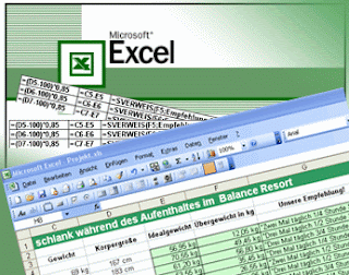
While working with formulas in Excel, you may feel the need to store and protect so that no change when you want to use it again. How?

Actually it's easy, even you can hide it all. Here's how.

• At first, first block of cells you want to hide the formula.

• Select the "Format Cell", followed by clicking on the tab "Protection". Enable "Locked" to lock and "Hidden" to hide it, then click "OK".

• Ensure that other cells do not come unlocked so that any time you can change existing data (Locked inactive, because its default active Locked) is to block all the cells would not be locked. Remember, do not activate the Locked and Hidden.

• Select "Tools> Protection> Protect Sheet ...". Dialog box will appear "Protect Sheet". Enable "Contents", then type the password that will be used, ending with "OK". Dialog box will show "Confirm Password" to make sure. Type the same password again, then press "OK". Presto! The formula will disappear suddenly.

• To bring it up again, select "Tools> Protection> Unprotect Sheet ...". Enter the password, then click "OK". Tada! The formula will reappear.

Jika anda merasa artikel ini bermanfaat, silahkan lakukan vote ke Lintas Berita agar artikel ini bisa di baca oleh orang lain. Suported by : Start Sharing Not Selling